Strain Transfer Across Grain Boundaries
The strain transfer across grain boundaries can be defined by the four following mechanisms (see Figure 6) [51], [81], [91] and [66]:
direct transmission with slip systems having the same Burgers vector, and the grain boundary is transparent to dislocations (no strengthening effect) (Figure 6-a);
direct transmission, but slip systems have different Burgers vector (leaving a residual boundary dislocations) (Figure 6-b);
indirect transmission, and slip systems have different Burgers vector (leaving a residual boundary dislocations) (Figure 6-c);
no transmission and the grain boundary acts as an impenetrable boundary, which implies stress accumulations, localized rotations, pile-up of dislocations… (Figure 6-d).
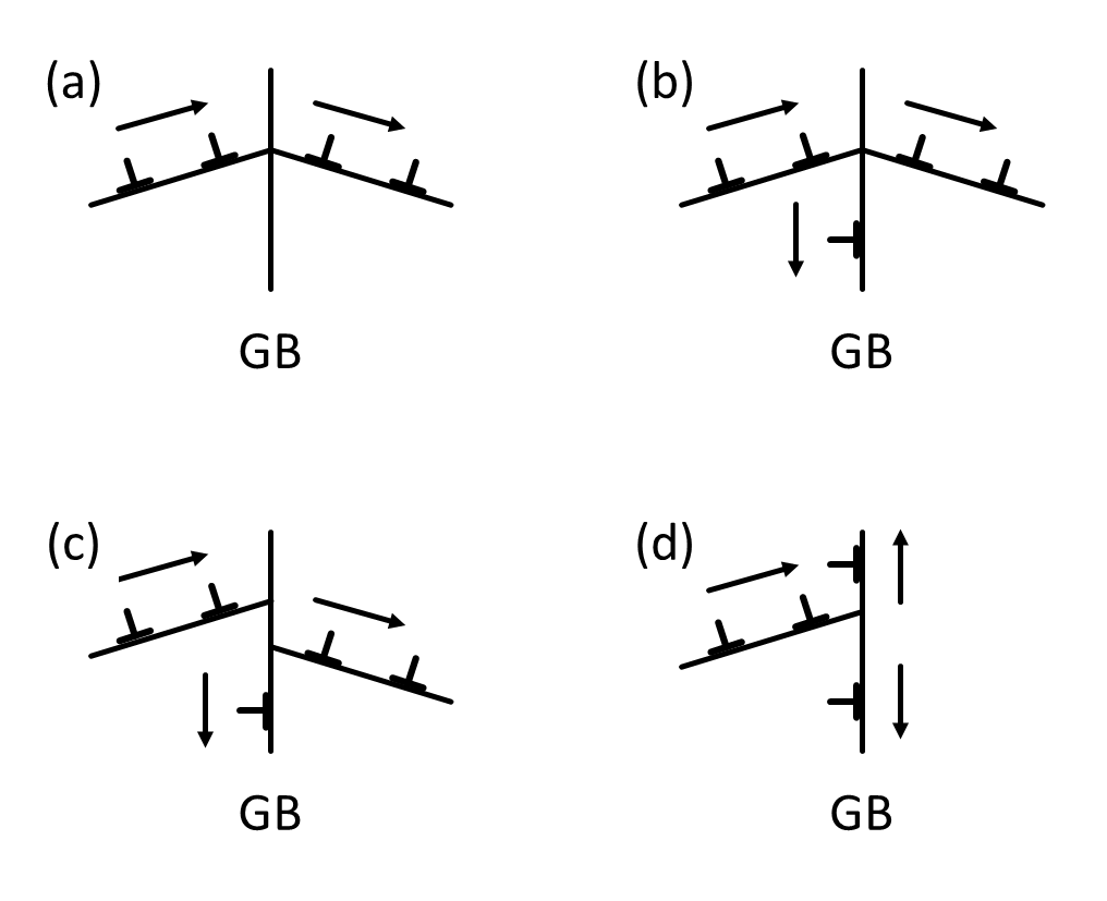
Figure 6 Possible strain transfer across grain boundaries (GB) from Sutton and Balluffi.
Several authors proposed slip transfer parameters from modelings or experiments for the last 60 years. A non-exhaustive list of those criteria is given in the next part of this work, including geometrical parameter, stress and energetic functions, and recent combinations of the previous parameters.
Note
Most of the time, following criteria are used to quantify slip transmission across grain boundaries in monophasic bicrystals. But in case of bimetal interfaces, it sounds that stress-based criteria are more relevant than geometrical criteria, given much higher stresses required for slip transmission [36].
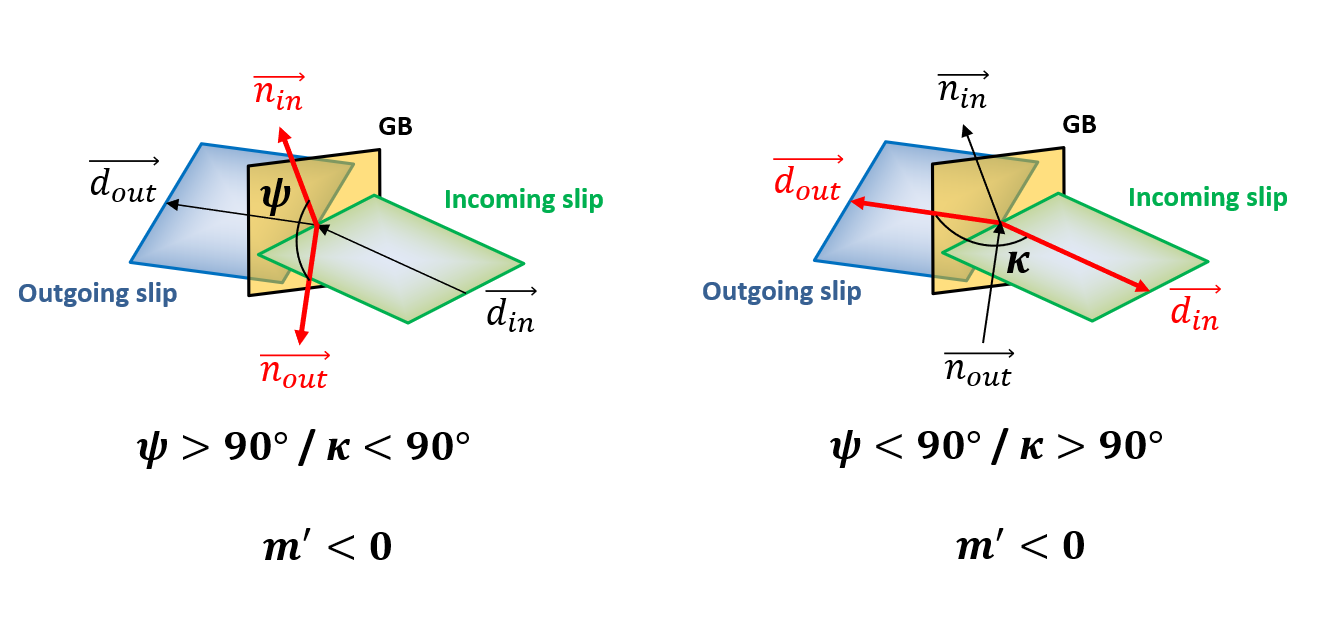
Geometrical Criteria
Based on numerous investigations of dislocation-grain boundary interactions, quantitative geometrical expressions describing the slip transmission mechanisms have been developed. A non-exhaustive list of geometrical criteria is detailed subsequently. The geometry of the slip transfer event is most of the time described by the scheme given Figure 7. \(\kappa\) is the angle between slip directions, \(\theta\) is the angle between the two slip plane intersections with the grain boundary, \(\psi\) is the angle between slip plane normal directions, \(\gamma\) is the angle between the direction of incoming slip and the plane normal of outgoing slip, and \(\delta\) is between the direction of outgoing slip and the plane normal of incoming slip. \(n\), \(d\) and \(l\) are respectively the slip plane normals, slip directions and the lines of intersection of the slip plane and the grain boundary. \(\vec b\) is the Burgers vector of the slip plane and \(\vec b_\text r\) is the residual Burgers vector of the residual dislocation at the grain boundary. The subscripts \(\text{in}\) and \(\text{out}\) refer to the incoming and outgoing slip systems, respectively.
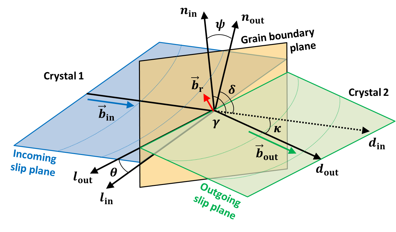
Figure 7 Geometrical description of the slip transfer.
\(N\) factor from Livingston and Chalmers in 1957 [53]
Many authors referred to this criterion to analyze slip transmission [32], [19], [34], [35], [73], [74], [48], [49], [17] and [84]. Pond et al. proposed to compute this geometric criteria for hexagonal metals using Frank’s method [65].
The Matlab function used to calculate the N factor is: N_factor.m
\(LRB\) factor from Shen et al. in 1986 [73] and [74]
The original notation of this \(LRB\) factor is \(M\), but unfortunately this notation is often used for the Taylor factor [11]. Pond et al. proposed to compute this geometric criteria for hexagonal metals using Frank’s method [65]. Recently, Spearot and Sangid have plotted this parameter as a function of the misorientation of the bicrystal using atomistic simulations [80].
[47], [48], [49], [17], [42], [43], [2], [28], [29] and [75] mentioned in their respective studies this geometrical parameter as a condition for slip transmission.
The inclination of the grain boundary (\(\beta\)) is required to evaluate this factor and the \(LRB\) or \(M\) factor should be maximized.
The Matlab function used to calculate the LRB factor is: LRB_parameter.m
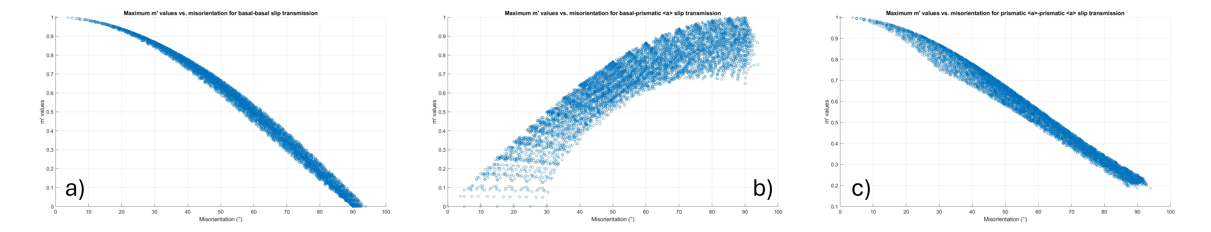
\(m'\) parameter from Luster and Morris in 1995 [54]
Many authors found that this \(m'\) parameter, which takes into account the degree of coplanarity of slip systems, is promising to predict slip transmission [87], [90], [13], [10], [11] , [30], [85], [31] and [58]. Both \(m'\) and \(LRB\) can be easily assessed in computational experiments [11]. This \(m'\) factor should be maximized (\(1\) means grain boundary is transparent and \(0\) means grain boundary is an impenetrable boundary). Negative values for \(m'\) factor means that slip plane direction or slip plane normals are in different directions. A value of \(-1\) for the \(m'\) factor means that grain boundary is transparent, but slip transmission may not occur, given different slip directions.
The Matlab functions used to calculate all maximum slip transmission parameters values as a function of bicrystal misorientation, are in the following folder: plot_Max-mprime_values_VS_misor
This factor is equal to \(0\), when grain boundary is transparent to dislocations. This implies \(m'\) parameter equal to \(1\) (slips perfectly aligned).
The Matlab function used to calculate the m’ parameter is; mprime.m
- \(\vec b_\text r\) the residual Burgers vector [56], [12], [51], [52], [16], [49] and [17].
- (13)¶\[\vec b_\text{r} = \vec g_\text{in}\cdot\vec b_\text{in} - \vec g_\text{out}\cdot\vec b_\text{out}\]
The magnitude of this residual Burgers vector should be minimized.
Shirokoff et al., Kehagias et al., and Kacher et al. used the residual Burgers vector as a criterion to analyse slip transmission in cp-Ti (HCP) [76], [42], [43] and [39], Lagow et al. in Mo (BCC) [45], Gemperle et al. and Gemperlova et al. in FeSi (BCC) [28] and [29], Kacher et al. in 304 stainless steel (FCC) [38], and Jacques et al. for semiconductors [37].
Misra and Gibala used the residual Burgers vector to analyze slip across a FCC/BCC interphase boundary [57].
Patriarca et al. demonstrated for BCC material the role of the residual Burgers vector in predicting slip transmission, by analysing strain field across GBs determined by digital image correlation [64].
As explained by Abuzaid et al., to give a physical meaning of the residual Burgers vector calculation, it is important to check the sign of the inner product between the slip direction and the vector defining the normal to the grain boundary plane. A positive result for such inner product indicates that the slip direction is incident relative to the grain boundary and a negative inner product indicates that transmission occurs [1].
The Matlab function used to calculate the residual Burgers vector is: residual_Burgers_vector.m
The misorientation or disorientation (\(\Delta g\) or \(\Delta g_\text d\)) [3], [15] and [90]
It has been observed during first experiments of bicrystals deformation in 1954, that the yield stress and the rate of work hardening increased with the orientation difference between the crystals [3] and [15].
Some authors demonstrated a strong correlation between misorientation between grains in a bicrystal and the grain boundary energy through crystal plasticity finite elements modelling and molecular dynamics simulations [81], [55], [50], [5], [69] and [70]. Some authors studied the stability of grain boundaries by the calculations of energy difference vs. misorientation angle through the hexagonal c-axis/a-axis [26].
The misorientation and disorientation equations are given in the crystallographic properties of a bicrystal.
The Matlab function used to calculate the misorientation angle is: misorientation.m
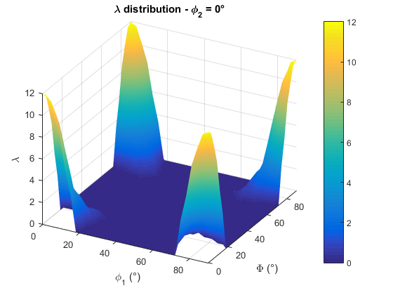
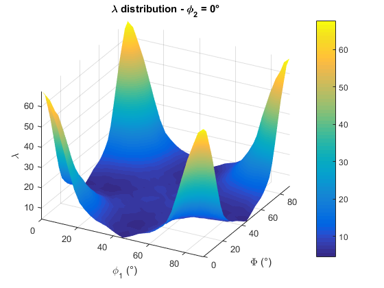
\(\lambda\) function from Werner and Prantl in 1990 [88]
With this function, slip transmission is expected to occur only when the angle \(\psi\) between slip plane normal directions is lower than a given critical value (\(\psi_c = 15°\)) and the angle \(\kappa\) between slip directions is lower than a given critical value (\(\kappa_c = 45°\)).
The Matlab function used to calculate the \(\lambda\) function is: lambda.m
The authors proposed to plot pseudo-3D view of the \(\lambda\) map (see Figures 5 and 6) using the following equation [88]:
(16)¶\[\lambda = \sum\limits_{\alpha=1}^N \sum\limits_{\beta=1}^N \cos\left(\frac{90°}{\psi_c}\arccos(\vec n_{\text{in},\alpha} \cdot \vec n_{\text{out},\beta})\right)\cos\left(\frac{90°}{\kappa_c}\arccos(\vec d_{\text{in},\alpha} \cdot \vec d_{\text{out},\beta})\right)\]With \(N\) the number of slip systems for each adjacent grains.
The Matlab function used to plot pseudo-3D view of the the \(\lambda\) function is: lambda_plot_values.m
This function is modified by Beyerlein et al., using the angle \(\theta\) between the two slip plane intersections with the grain boundary, instead of using the angle \(\psi\) between the two slip plane normal directions [9].
The Matlab function used to calculate the modified \(\lambda\) function is: lambda_modified.m
Stress Criteria
Schmid Factor (\(m\)) [68], [71] and [1]
The Schmid’s law can be expressed by the following equation:
\(\sigma\) is an arbitrary stress state and \(\tau^i\) the resolved shear stress on slip system \(i\). \({S_0}^i\) is the Schmid matrix defined by the dyadic product of the slip plane normals \(\vec n\) and the slip directions \(\vec d\) of the slip system \(i\). The Schmid factor, \(m\), is defined as the ratio of the resolved shear stress \(\tau^{i}\) to a given uniaxial stress.
Knowing the value of the highest Schmid factor of a given slip system for both grains in a bicrystal, Abuzaid et al. [1] proposed the following criterion:
(21)¶\[m_\text{GB} = m_\text{in} + m_\text{out}\]The subscripts \(\text{GB}\), \(\text{in}\), and \(\text{out}\) refer to the grain boundary, and the incoming and outgoing slip systems, respectively. This GB Schmid factor (\(m_\text{GB}\)) factor should be maximized.
The Matlab function used to calculate the Schmid factor is: resolved_shear_stress.m
Generalized Schmid Factor (\(GSF\)) [68] and [11]
The generalized Schmid factor, which describes the shear stress on a given slip system, can be computed from any stress tensor \(\sigma\) based on the Frobenius norm of the tensor.
(22)¶\[GSF = \vec d \cdot g \sigma g \cdot \vec n\]\(\vec n\) and \(\vec d\) are respectively the slip plane normals and the slip directions of the slip system. The \(g\) is the orientation matrix for a given crystal.
The Matlab function used to calculate the generalized Schmid factor is: generalized_schmid_factor.m
Resolved Shear Stress (\(\tau\)) [47], [48], [49], [17], [45], [10], [22], [23] and [24]
The resolved shear stress \(\tau\) acting on the outgoing slip system from the piled-up dislocations should be maximized. This criterion considers the local stress state.
The resolved shear stress on the grain boundary should be minimized.
For Shi and Zikry, the ratio of the resolved shear stress to the reference shear stress of the outgoing slip system (stress ratio) should be greater than a critical value (which is approximately 1) [75].
For Li et al. and Gao et al. the resolved shear stress acting on the incoming dislocation on the slip plane must be larger than the critical penetration stress. From the energy point of view, only when the work by the external force on the incoming dislocation is greater than the summation of the GB energy and strain energy of GB dislocation debris, it is possible that the incoming dislocation can penetrate through the GB [50] and [27].
It is possible to assess the shear stress from the geometrical factor \(N\) (Livingston and Chamlers):
(23)¶\[\tau_{\text{in}} = \tau_{\text{out}} * N\]Where \(\tau_{\text{out}}\) is the shear stress at the head of the accumulated dislocations in their slip plane and \(\tau_{\text{in}}\) is the shear acting on the incoming slip system [53], [34] and [35].
The Matlab function used to calculate the resolved shear stress is: resolved_shear_stress.m
Combination of Criteria
Geometrical function weighted by the accumulated shear stress or the Schmid factor [11]:
Bieler et al. proposed to weight slip transfer parameters by the sum of accumulated shear \(\gamma\) on each slip system, knowing the local stress tensor. From a crystal plasticity simulation, the accumulated shear is the total accumulated shear on each slip system for a given integration point. This leads to the following shear-informed version of a slip transfer parameter:
(24)¶\[m_{\gamma}^{'} = \frac{\sum_{\alpha} \sum_{\beta} m_{\alpha\beta}^{'} \left(\gamma^{\alpha} \gamma^{\beta} \right)}{\sum_{\alpha} \sum_{\beta} \left(\gamma^{\alpha} \gamma^{\beta} \right)}\](25)¶\[LRB_{\gamma} = \frac{\sum_{\alpha} \sum_{\beta} LRB_{\alpha\beta}^{'} \left(\gamma^{\alpha} \gamma^{\beta} \right)}{\sum_{\alpha} \sum_{\beta} \left(\gamma^{\alpha} \gamma^{\beta} \right)}\](26)¶\[s_{\gamma} = \frac{\sum_{\alpha} \sum_{\beta} s_{\alpha\beta}^{'} \left(\gamma^{\alpha} \gamma^{\beta} \right)}{\sum_{\alpha} \sum_{\beta} \left(\gamma^{\alpha} \gamma^{\beta} \right)}\](27)¶\[s = \cos(\psi) \cdot \cos(\kappa) \cdot \cos(\theta)\]The Matlab function used to calculate the \(s\) function is: s_factor.m
Similarly, the \(m^{'}\) parameter can be weighted using the Schmid factor \(m\) on each slip system as a metric for the magnitude of slip transfer:
(28)¶\[m_{GSF}^{'} = \frac{\sum_{\alpha} \sum_{\beta} m_{\alpha\beta}^{'} \left(m^{\alpha} m^{\beta} \right)}{\sum_{\alpha} \sum_{\beta} \left(m^{\alpha} m^{\beta} \right)}\]In 2016, Tsuru et al. proposed a new criterion, based on the \(N\) factor, for the transferability of dislocations through a GB that considers both the intergranular crystallographic orientation of slip systems and the applied stress condition [83].
Relationships between slip transmission criteria
Some authors proposed to study relationships between slip transmission criteria [30] and [86]. Thus, it is possible to find in the literature the \(m'\) parameter plotted as a function of the Schmid factor or the misorientation angle. Such plots based on experimental values allow to map slip transmissivity at grain boundaries for a given material.
Slip transmission parameters implemented in the STABiX toolbox
Slip transmission parameter |
Function |
Matlab function |
Reference |
|---|---|---|---|
Misorientation angle (FCC and BCC materials) (\(\omega\)) |
\(\omega = cos^{-1}((tr(\Delta g)-1)/2)\) |
||
C-axis misorientation angle (HCP material) (\(\omega\)) |
|||
\(N\) factor from Livingston and Chamlers |
\(N = \cos(\psi)\cdot\cos(\kappa) + \cos(\gamma)\cdot\cos(\delta)\) |
||
\(LRB\) factor from Shen et al. |
\(LRB = \cos(\theta)\cdot\cos(\kappa)\) |
||
\(m'\) parameter from Luster and Morris |
\(m' = \cos(\psi)\cdot\cos(\kappa)\) |
||
residual Burgers vector (\(\vec b_\text{r}\)) |
\(\vec b_\text{r} = g_\text{in}\cdot\vec b_\text{in} - g_\text{out}\cdot\vec b_\text{out}\) |
||
\(\lambda\) function from Werner and Prantl |
\(\lambda = \cos(\frac{90° \psi}{\psi_c})\cos(\frac{90° \kappa}{\kappa_c})\) |
||
Resolved Shear Stress (\(\tau^{i}\)) / Schmid Factor |
\(\tau^{i} = \sigma : {S_0}^{i}\) with \({S_0}^{i} = d \otimes n\) |
||
Grain boundary Schmid factor |
\(m_\text{GB} = m_\text{in} + m_\text{out}\) |
||
Generalized Schmid Factor (\(GSF\)) |
\(GSF = d \cdot g \sigma g \cdot n\) |
Slip and twin systems implemented in the STABiX toolbox
List of slip and twin systems for FCC phase material used in STABiX and DAMASK - FCC.
List of slip and twin systems for BCC phase material used in STABiX and DAMASK - BCC.
List of slip and twin systems for HCP phase material used in STABiX and DAMASK - HCP.
Effects of number of slip systems on slip transmission
The effects of the number of slip systems on the transmission criteria can be plotted and analyzed to discuss plastic deformation occuring in metals and alloys. Such approach has been discussed by Ogasawar et al. [60] and a plot in parallel of this work using the STABIX toolbox is given as an example with Figure 9.